
Query Language
In computer science, languages are set of grammatical rules for instructing a computer or computing device to perform specific tasks. Similarly Query Language is used specifically to instruct or communicate with database for retrieving or processing of data. Query Languages are also called as Data Query Languages (DQL).
Typically, this language is similar and close to the simple English language. it’s not really a programming language. Its sole purpose is to access, create, and manipulate data in databases. While it does contain basic programming necessities such as loops, simple (in)equality/logical operators, and if/else control flow, it cannot be used for anything other than data manipulation. Thus, it’s not considered a real or 100% programming language; rather, it’s more of an ‘extension’ that we can utilise in other languages. As you know there are many types of Database models like Relational DB , Object Oriented DB etc. So there are different Query languages for different Database models. E.g SQL for Relational Databases, OQL for Object Oriented Databases etc. In this post we will concentrate on Languages and its related concepts for Relational Databases.
Query Languages for RDBMS
There are mainly two types of query languages for Relational Database Management System.
Procedural QL (Relational Algebra)
In this language, the programmer needs to define two things. One is What to do and second is How to do. I.e you have to always specify the details of the query operation such as opening and closing tables, loading and searching indexes, or flushing buffers and writing data to filesystems, sequence of query operations to get the desired output. This language is based on concepts of Relational Algebra.
Non-Procedural QL (Relational Calculus)
Here you don’t need to specify any details about the operation. You just need to specify what to do and DBMS software will take care rest of it. This is based on concept of Relational Calculus.
Importance of Relational Algebra/Calculus
Well, let’s do some analyze first if it is really required to learn these basic old things to gain some deep knowledge in modern world query language like SQL. Doesn’t it seem like learning how to formulate query-like expressions in relational algebra is a traditional part of many, perhaps most, “Introduction to Databases” courses only. Does it seem to you that formulating expressions in relational algebra is basically the same as formulating queries in SQL and that much the same thought processes. In particular, do you think you don’t see that knowing these concepts makes it easier to write SQL queries or vice-versa.
Actually when Codd defined the relational model he defined a set of operators which could be applied to relations (Tables). For example, in integer algebra we know that addition and multiplication are associative. So that we can change the grouping of operands which not change the result.
a + ( b + c ) = ( a + b ) + c
Similarly, in relational algebra or calculus we know that natural join is associative and thus know that A join B join C can be executed in any order. These properties and laws create the power to re-write query formulations and be guaranteed to get the same results. Thus if you have formulated a query one way and are getting poor performance, you have the skills to formulate it in a different way and know it has the same semantics.
It was Leonardo da Vinci who said:
He who loves practice without theory is like the sailor who boards ship without a rudder and compass and never knows where he may cast.
Now we will go through the details of Relational Algebra and Relational Calculus. One more thing to remind. As we know, Algebra or Arithmetic are the branch of Mathematics to deal with number systems, similarly these concepts are to deal with Database systems. In mathematics, say we are adding two numbers. We call those numbers as operands and the addition (+) as operator. Similarly in relational algebra or calculus we have many operators which we will discuss below. Tables/Relations are called as operands here.
Relational Algebra
Note : Relational Algebra is not same as Relation Algebra. So don’t be confused.
In relational algebra an operator can be either unary or binary. They accept relations (tables) as their input and yield relations (tables) as their output. Also note that the output table will have no name and it will not contain any duplicate row.
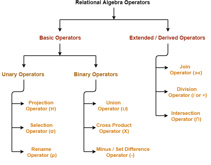
There are 6 fundamental or basic operators in relational algebra as follows :
- Select (σ)
- Project (∏)
- Union (∪)
- Set different (−)
- Cartesian product (Χ)
- Rename (ρ)
And some operators are derived from the above basic operators which we call derived operator:
- Join
- Intersection
- Division
Let’s discuss on those operators one by one with example. Say a table named as Student as follow.
| ID | Name | Course |
| 1 | A | CS |
| 2 | B | MECH |
| 3 | A | EEE |
( Student )
Select (σ)
This is an unary operator. It means it can take only one table as input. It can retrieve one or multiple rows from the input table which satisfy the given condition (Predicate). Connectors like and (∧), or (∨), not (!), = (-), ≠, ≥, < , >, ≤ can be used inside the condition.
Selection operator always selects the entire tuple. It can not select a section or part of a tuple. Degree of the relation from a selection operation is same as degree of the input relation. The number of rows returned by a selection operation is obviously less than or equal to the number of rows in the original table. Thus, Minimum Cardinality = 0, Maximum Cardinality = |R|
Notation : σ(condition )(Table Name)
Example : σ( ID = 2)(Student)
Output :
| ID | Name | Course |
| 2 | B | MECH |
Note: Selection operator is commutative in nature i.e. σ A ∧ B (R) = σ B ∧ A (R) . See this video for more complex example
Project (∏)
This is also an unary operator. It can retrieve one or more desired columns that satisfy a condition or predicate. If you want to get multiple columns you can write those separated by comma like below example.
Notation : ∏( column names )(Table Name)
Example : ∏( id, course )(Student)
Output :
| ID | Course |
| 1 | CS |
| 2 | MECH |
| 3 | EEE |
See this video for more example. Some more complex examples here and here.
Union (∪)
It performs binary union between two given tables like SET theory union among two sets. All the rules of set theory union will be applicable here also. Note two tables must be union compatible i.e they should have the same number of attributes and the attribute domains (types of values accepted by attributes) of both the relations must be compatible.
Notation : r ∪ s , where r and s both are two different tables not set of course.
Example : ∏ author (Books) ∪ ∏ author (Articles)Output : Projects the names of the authors who have either written a book or an article or both.
Set difference (−)
The result of set difference operation is tuples, which are present in one relation but are not in the second relation. This is also same as SET difference.
Notation : r − s ( Finds all the tuples that are present in r but not in s )
Example : ∏ author (Books) − ∏ author (Articles)Output : Provides the name of authors who have written books but not articles.
Must watch this video for union and difference example.
Cartesian product (Χ)
I would suggest to must watch this video to understand the Cartesian product and its use. See this for complex example.
Rename (ρ)
The results of relational algebra are also relations but without any name. The rename operation allows us to rename the output relation. ‘rename’ operation is denoted with small Greek letter rho ρ.
Notation : ρ desired_table_name (expression_to_be_evaluated)
Example : ρ x (E)
Output : Where the result of expression E is saved with name of x.
Join (⋈)
You already know doing Cartesian product between two tables we can get all the possible combination of relations. If you have already watched the videos related to Cartesian Product and some complex examples given above, you might have understood that Cartesian Product also joins two tables. But the resulting tables may contain some unnecessary or invalid rows which you need to filter out using Select operator. Isn’t it an extra step always you have to perform after every Cartesian Product? That is why there are some derived operators like Join which minimizes those extra steps and give you the direct result. Infact Join is not doing any magic. Internally it also performs those extra steps (Cross product and then Selection based on some conditions), but you don’t see it. There are mainly two types of Joins and again they are also further classified based on their conditions.
Note: When you will have to retrieve some data from two different tables you can easily get the results using JOIN at that time. But I never said you that you can’t use Join for a single table. That is actually a Self join which we will discuss in SQL.
Inner Joins
- Theta join
It combines tuples (rows) from different relations provided they satisfy the given condition. The Join condition is denoted by the symbol θ. It can use all kinds of comparison operators ( =, >, <. <=, >=, <>).Notation : R1 ⋈θ R2 (Where R1 and R2 are two relations having attributes (A1, A2, .., An) and (B1, B2,.. ,Bn) such that the attributes don’t have anything in common, that is R1 ∩ R2 = Φ ) Example :
student SID Name Std 101 Alex 10 102 Maria 11 subjects Class Subject 10 Math 10 English 11 Music 11 Sports Output :STUDENT ⋈(student.Std = subject.Class) SUBJECT SID Name Std Class Subject 101 Alex 10 10 Math 101 Alex 10 10 English 102 Maria 11 11 Music 102 Maria 11 11 Sports - Equi join
When theta join uses only equality comparison operator inside conditions, we can call it Equi join. The above example can also be called as Equi join. - Natural join
It does not utilize any of the comparison operator. Here the condition is that the attributes(Column) should have same name and domain. We can perform a Natural Join only if there is at least one same common that exists between two relations. Internally, it forms the cartesian product of two tables, performs selection forming equality on those attributes that appear in both relations and eliminates the duplicate attributes.Courses CID Course Dept 01 Database CS 02 Mechanics ME 03 Electronics EE HoD Dept Head CS Alex ME Maya EE Mira Courses ⋈ HoD Dept CID Course Head CS 01 Database Alex ME 02 Mechanics Maya EE 03 Electronics Mira
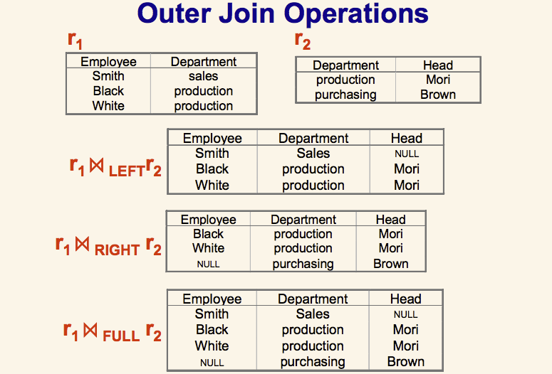
Outer Joins
Though both inner and outer joins include rows from both tables when the match condition is successful, they differ in how they handle a false match condition. Inner joins don’t include non-matching rows; whereas, outer joins do include them.
- Left outer join (Video link)
- Right outer join (Video Link)
- Full outer join (Video Link)
Division
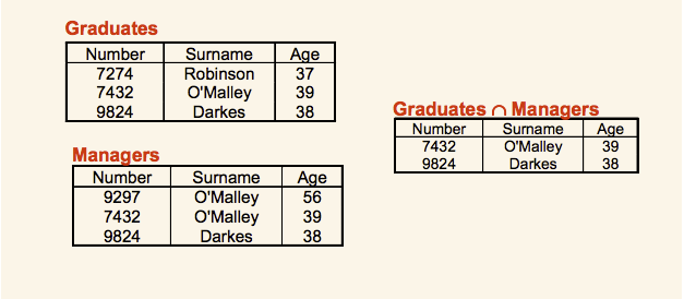
Intersection
Intersection on two relations R1 and R2 can only be computed if R1 and R2 are union compatible ( i.e both relations should have same number of attributes(columns) and corresponding attributes in two relations have same domain). Intersection operator when applied on two relations as R1∩R2 will give a relation with tuples(rows) which are both in R1 and R2.
Relational Calculus
Contrary to Relational Algebra which is a procedural query language to fetch data and which also explains how it is done, Relational Calculus in non-procedural query language and has no description about how the query will work or the data will b fetched. It only focuses on what to do, and not on how to do it.
Relational Calculus exists in two forms:
- Tuple Relational Calculus (TRC)
- Domain Relational Calculus (DRC)
Tuple Relational Calculus (TRC)
In tuple relational calculus, we work on filtering tuples based on the given condition.
Syntax: { T | Condition }
In this form of relational calculus, we define a tuple variable, specify the table(relation) name in which the tuple is to be searched for, along with a condition.
We can also specify column name using a . dot operator, with the tuple variable to only get a certain attribute(column) in result.
A lot of information, right! Give it some time to sink in.
A tuple variable is nothing but a name, can be anything, generally we use a single alphabet for this, so let’s say T is a tuple variable.
To specify the name of the relation(table) in which we want to look for data, we do the following:
Relation(T), where T is our tuple variable.
For example if our table is Student, we would put it as Student(T)
Then comes the condition part, to specify a condition applicable for a particluar attribute(column), we can use the . dot variable with the tuple variable to specify it, like in table Student, if we want to get data for students with age greater than 17, then, we can write it as,
T.age > 17, where T is our tuple variable.
Putting it all together, if we want to use Tuple Relational Calculus to fetch names of students, from table Student, with age greater than 17, then, for T being our tuple variable,
T.name | Student(T) AND T.age > 17
Domain Relational Calculus (DRC)
In domain relational calculus, filtering is done based on the domain of the attributes and not based on the tuple values.
Syntax: { c1, c2, c3, …, cn | F(c1, c2, c3, … ,cn)}
where, c1, c2… etc represents domain of attributes(columns) and F defines the formula including the condition for fetching the data.
For example,
{< name, age > | ∈ Student ∧ age > 17}
Again, the above query will return the names and ages of the students in the table Student who are older than 17.
SQL (The real Implementation)
Above you read all the mathematical concepts to query a Relational Database. But in real world SQL was the first commercial language implemented in 1970 based on above mathematical concepts by IBM. This version, initially called SEQUEL (Structured English Query Language), was designed to manipulate and retrieve data stored in IBM’s original quasi-relational database management system. The acronym SEQUEL was later changed to SQL because “SEQUEL” was a trademark of the UK-based Hawker Siddeley Dynamics Engineering Limited company.
It is actually based on both Relational Algebra and Calculus (TRC). However it is loosely depends upon Relational Algebra and more on Relational Calculus. So we often call SQL is a non-procedural language. Users describe in SQL what they want to do, and the SQL language compiler automatically generates a procedure to navigate the database and perform the desired task. I had previously also mentioned that SQL is not purely based on Relational Model. It is actually a hybrid and high end language.
SQL deviates in several ways from its theoretical foundation, the relational model and its tuple calculus. In that model, a table is a set of tuples, while in SQL, tables and query results are lists of rows: the same row may occur multiple times, and the order of rows can be employed in queries (e.g. in the LIMIT clause).